

In increasingly competitive basketball conferences, professional teams are looking to get an edge on analysis-based games. March 31, 2018By Peter Scharf_______It is Thursday March 30th and the opening day of the regular season for the Philadelphia Phillies and I am as least interested as I have been in years. Not because the Phillies are coming off a season where they posted one of the worst records in the league, not because most of the talent is not developed, and not because I have moved on to a win-now team. It is primarily because 1: Schoolwork in my final semester has slowly rotted away at my soul, 2: I have spent the last month or so taking my statistics skills into basketball, and 3: The Philadelphia 76ers are scorching the Earth that is the Eastern Conference. Basically, the Sixers, once the laughing stock of the NBA, have dominated and secured a playoff spot.With the Sixers advancing on analysis-based basketball and being snowed in at my Philadelphia home during Spring Break, I was inspired to build an NBA model that led to this post. To start, I will look into the game theory of basketball that the Sixers and a few other teams utilize.Maximizing Expected Shot ValueImagine a basketball court as some sort of weird matrix. Each area on the court has two components that go into the expected shot value, the worth of the shot and the percentage a shot from a certain area goes in. As a basketball player, or a coach coming up with a game plan, it would be desirable to shoot shots that maximize the expected shot value of a given situation.Up until the 1980 season in the NBA, the only way to do this was to get close to the basket. Big men dominated and much of the basketball action was closer to the rim. In 1980 things changed, the 3-point line was implemented. This made shots beyond its arc worth 0.5 times more than a standard shot.At first its usage was mainly as a gimmick.Today, teams are taking more threes than ever. As of this piece’s writing, the Houston Rockets are set to be the first team to ever take more threes than twos. The takeover of the three-point line has primarily been influenced by analytic based GMs and coaches maximizing expected shot value.Going back to the example of the basketball court matrix, the percentage of shots that go in decays the further you get away from the basket. Slam dunks, the closest shots, go in at near 100% clips. Long two’s and three’s dip under 50%. Basically, the further you get away from the basket the lower the percentage of shots that go in. This makes sense both statistically and in a “common sense” way. The further you are from the basket the harder it is for the ball to go in. Now, enter the three-point line.Although the league average on a 3-point shot is only 36%, the shot is worth 3 points and thus 3*.36=1.08 which is the expected shot value. Now imagine you are moving in towards the basket. Once you get inside 22 feet, you are no longer shooting a shot worth 3 points, however, the field goal percentage goes up.Shots from 15ft-22ft from the basket are worth two and go in 44% of the time. This leads to an expected shot value of 2*.44=.88, lower than taking a three. Moving even closer to the basket, the shot percentage goes up again. From 10ft-15ft out (approximately inside the distance from halfway to the foul line to the foul line), the field goal percentage climbs to nearly 50%.The expected shot value is approximately 1. Going on, 6ft-10ft’s expected shot value is 0.55*2=1.10, and under the basket to 6ft results in a 0.66*2= 1.32. Technically under the basket is only 0.82*2= 1.64. So, what happened here? Three-point shots are worth more than one expected point, and not until you get within the foul line are shots worth more than 1 expected point. Being that defenses make it more difficult to get to the basket, often times it is a best response to not dribble in towards the hoop, but rather step back and take a three.Across a season with 1000s of shots being taken, the law of averages sways in your favor. The dominant strategy ends up being a mixed strategy of taking shots underneath, in the in the red and blue zones, as well as beyond the three-point arc in the purple. The green and yellow are not best response shots because if you can not get the ball to the red or blue, you are better off passing it behind you and taking a three.So what does a game plan look like following this strategy? Basically, shooters are posted on the outside around the three-point line and a big man is posted up underneath the basket. The point guard brings the ball up and attempts to get the ball to the big man as shots under 10ft are worth 1.32+ and if that is unavailable, he passes to one of the shooters for an expected shot value of 1.08. Following this plan of maximizing expected shot value, the team should average over 100 points per possession. Here is what it looks like in action.This is a screenshot of the Sixer’s March 19 win over the Hornets.
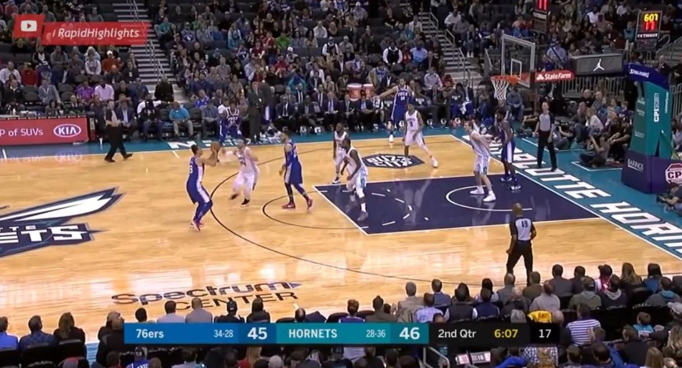 The Sixers, in blue, have all their offensive scorers located in areas that maximize expected shot value. Dario Saric, the player just beyond the arc taking the shot, Robert Covington, Saric’s left, and JJ Reddick, far corner, are all ready shooters with a high expected shot value because they are beyond the three. In this specific case, Saric, Reddick, and Covington are elite shooters and all shoot above 40% from three making their expected shot value 0.40*3=1.2. The other Sixer, Amir Johnson, is directly underneath the basket anticipating a pass or a rebound for another shot with a high expected value. The only Sixer not in a maximized space is Ben Simmons who brought the ball up to the foul line then turned around a passed it to Saric because the expected value of a foul line shot from Simmons is less than a Saric three.Philadelphia 76er’s former GM Sam Hinkie realized this as well. When selecting players in the draft or through transactions with other teams, he picked either big men or shooters. The plan was to run a maximized offense for the next 10 years. While Sam Hinkie is no longer GM of the Philadelphia 76ers, his selected shooters in Robert Covington and Dario Saric as well as big men in Joel Embiid and Richaun Holmes continue to run this analytic based offense.
 Former Sixers GM Sam Hinkie talks with a young Joel Embiid shortly after his drafting. Using Econometrics to Forecast Basketball Games (and doing well)As evident by the fact that his name gets dropped in nearly every one of my blogs, I am a huge admirer of Nate Silver. Particularly how he takes economics and statistics and applies them to areas typically outside the field. In the area of sports, Nate Silver has shifted forecasting away from betting lines and ESPN “analysts” and more towards a quantitative and probabilistic approach. I figured if Nate Silver can do it, I can get close.Basketball seemed like the easiest sport to start forecasting. Looking at the top records in the league shows that the best teams generally win 70%-80% of their games. Compare this to a sport like baseball where teams are more even and the best team only wins 63% of their games. So essentially, basketball has more skill involved and less randomness, more signal to capture and less noise.At my aid are my new-found skills in R and enrollment in ECON483 Economic Forecasting (I highly recommend taking this course). I spent the first few days of my Spring Break gathering data and crunching numbers. Looking for patterns between wins, points and general basketball statistics. I began to diverge into two types of basketball forecasting, macroforecasting and microforecasting. Macroforecasting pertains to season long play. How many wins will the team have? Where will they place in their conference? Which team will score the most points this season? Macroforecasting does this very well.
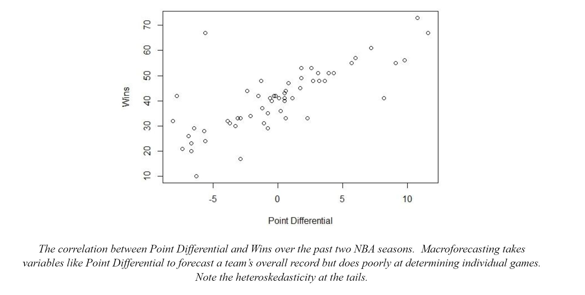 For individual games, the macroforecasting approach was not effective. I realized this when I was explaining my research to a friend and he responded “Who cares?, I just want to know who wins tonight!” .For game-by-game forecasting I needed to explore the microforecasting approach. This approach looks at the scoring and defense of the two teams in a game and determines in outcome, this approach ends up being much more difficult.To model an individual game, be careful about what stats you use. Player stats are often measured in three different ways: per game, per 100 possessions, and per 36 minutes. It is important to focus on per game stats. Per possession and per minute stats are better on player specific statistics but on a whole team they are a poor measure. Remember, every team only control the pace when they are on offense. Stats like offensive efficiency and defensive efficiency can be skewed by fast or slow offenses in an actual game format.My microforecasting model continues to be refined but it looks something like this:The result of the game is Yv - Yh where Y is the predicted points for each team. If this number is positive, the visitor wins. If it is negative it is a home victory. Y is composed of:
 Where y is the predicted points, Ha is a dummy (binary) variable that is activate for the home team because across 2056 games a clear home field advantage was observed, B is an adjusted average of points scored per game, Dj is the defense added points of the opposition (good defenses this number is negative because they take away and bad defenses have this as a positive number. This number can also be influenced by how fast the opposing team’s offense runs.), and E is an error term. Numbers get rounded down to whole numbers because you cannot score half points in basketball. My actual running model is of course more complicated than this, but this equation accounts for most of it.As an example, let's use the Friday March 30th, 2018 7:30PM game with the Philadelphia 76ers facing off against the Atlanta Hawks. The Sixers forecasted score is:
 For the Hawks it is:
 Thus, the forecasted result is:
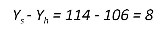 The model forecasts a Sixers, the visiting team, victory by plus 8. The actual game was much lower scoring than anticipated, particularly because the Sixers played their worst players in the 4th quarter to rest the starters for the playoffs, and the final score was 101-91. The Sixers won by 10 and the residual between the forecast and the actual score is -2. Although not perfect, sports are volatile and getting this close is impressive.To run this regression in programs like STATA and R, treat opposing defenses like seasonality. This will treat the opposing defenses like dummy variables and apply them when the team name is equal to a certain character value. To visualize the effect of opponent defense on score look at the plot below. It is the 76ers scores for each game plotted twice, to the left of the black line for unadjusted and to the right for adjusted. The red dashed lines are at 119 and 99 (within one standard deviation) and the green line is the Sixer’s B of 109. Although slightly, the right side of the black line is more correlated around the mean.
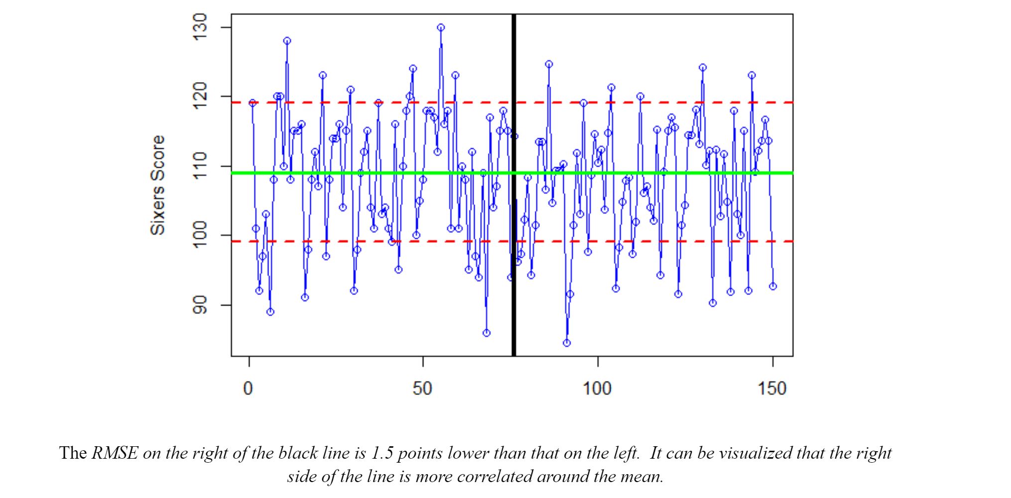 As a sports fan, using the stat and game theory skills I picked up in the classroom through the B.S. in Economics allows me to get involved with the game. I have become a more informed fan, despite only watching half of my home team’s games. I encourage anyone to apply statistics to an interest of theirs, it is surprisingly fun and gives new insights into that field._______ Author's Note: All statistical data comes from basketballreference.com All analysis and graphing was done using R within Rstudio or Microsoft Excel. For more information contact optimalbundle.psuea@psu.edu. Editor's Note: Minor changes have been made to the original version of this piece. Feature Image Credit: Public Domain